

SITCOMTN-158
WET-006 stacking with ComCam data#
This document compares two methods for wavefront estimation in the Rubin Observatory Active Optics System (AOS). The first, and currently default, method—referred to as pairing—involves fitting wavefronts to individual donut pairs and averaging the resulting Zernike coefficients. The second method, known as stacking, combines multiple individual donut images into a single stacked image prior to wavefront fitting, producing one set of Zernike coefficients per stacked image. For a high-level overview of the pairing and stacking approaches, see SITCOMTN-085.
Last verified to run: 04/24/2025
Versions:
lsst_distrib w_2025_16 (ext, cvmfs)
ts_wep v14.3.2
Imports#
import os
import sys
import numpy as np
import pandas as pd
from astropy.table import Table
from astropy.table import join
from astropy.time import Time, TimeDelta
from astropy.visualization import ZScaleInterval
from datetime import datetime, timedelta
from lsst.daf import butler as dafButler
from lsst.daf.butler import Butler
from lsst.summit.utils import ConsDbClient
from lsst.summit.utils.efdUtils import getEfdData, makeEfdClient
import lsst.summit.utils.butlerUtils as butlerUtils
from lsst.summit.utils.utils import computeCcdExposureId
from lsst.ts.wep.estimation import WfAlgorithmFactory, WfEstimator
from lsst.ts.wep.image import Image
from lsst.ts.wep.task.estimateZernikesBase import EstimateZernikesBaseConfig
from lsst.ts.wep.task.estimateZernikesDanishTask import EstimateZernikesDanishConfig
from lsst.ts.wep.task.estimateZernikesTieTask import EstimateZernikesTieConfig
from lsst.ts.wep.utils import (
    WfAlgorithmName,
    binArray,
    convertZernikesToPsfWidth,
    getCameraFromButlerName,
    getTaskInstrument,
    makeDense,
    makeSparse,
)
import matplotlib.pyplot as plt
from tqdm import tqdm

# Local import
sys.path.append("/sdf/data/rubin/user/scichris/WORK/sitcomtn-158/")
import run_stacking as rs  # noqa: E402

# Clear potentially problematic proxy env variable
#del os.environ["http_proxy"]
Illustrate stacking settings#
We use LSSTComCam Commissioning data collected during the period from October 21 to December 11, 2024 (total of 2474 defocal visits). From this dataset, we select 572 exposures that include at least nine donuts in the final accepted sample per detector. This ensures a minimum of nine individual Zernike estimates per detector, consistent with the selection criteria used in a previous study (SITCOMTN-156).
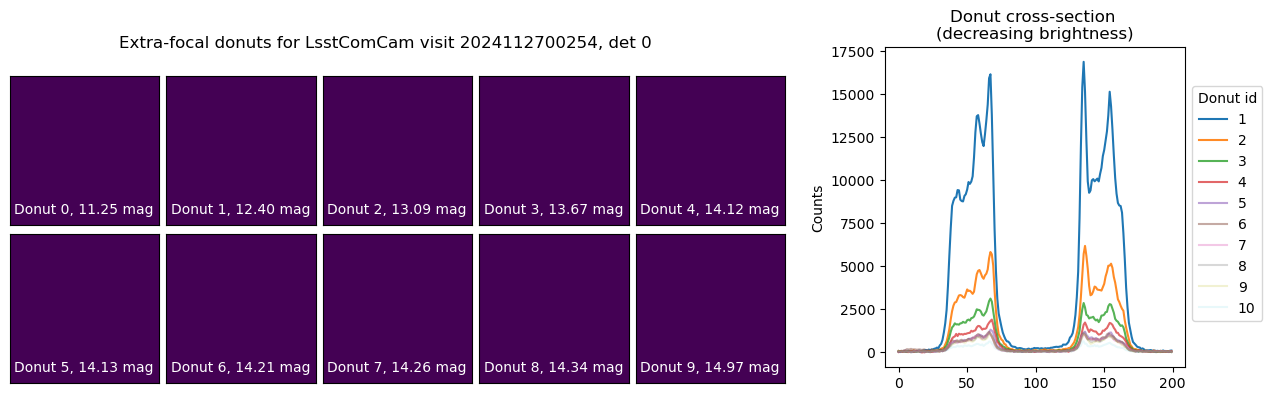
To begin, we illustrate the stacking process using donuts from a single visit. The left panel shows postage stamp cutouts from the post-ISR images, while the right panel displays the corresponding donut cross-sections. This visualization highlights how each donut contributes varying brightness and signal-to-noise to the final stacked average:
Nvisits = 1269
path_cwd = os.getcwd()
fname = os.path.join(path_cwd, f'u_scichris_aosBaseline_tie_danish_zernikes_tables_{Nvisits}.npy')
results_visit = np.load(fname, allow_pickle=True).item()


fname = os.path.join(path_cwd, 'u_scichris_aosBaseline_danish1_donutQualityTable_N_donuts_all_det_select_good_new.txt')
donutQualityTableSel = Table.read(fname, format='ascii')

results_visit_bin1 = {}
for visit in results_visit.keys():
    results_visit_bin1[visit] = {'tie1': results_visit[visit]['tie1'],
                                 'danish1': results_visit[visit]['danish1']
                                }
path_cwd = os.getcwd()
fname = os.path.join(path_cwd, f'u_scichris_aosBaseline_tie_danish_zernikes_tables_{Nvisits}_binning_1.npy')
np.save(fname, results_visit_bin1 , allow_pickle=True)
Show the donuts from one of the visits; note that just for illustration we’re showing the first few donuts, not necessarily the selected ones (that would be determined by the contents of donutQualityTable.
visit = 2024112700254
butler = Butler('/repo/main')
refs = butler.query_datasets('donutStampsExtra', collections = ['u/brycek/aosBaseline_step1a'],
                            where=f"instrument = 'LSSTComCam' and visit = {visit}",
                             detector=0
                           )
ref = refs[0]
detector = ref.dataId['detector']
# both intra and extra-focal donut stamps are stored under the extra-focal dataId
donutStampsExtra = butler.get('donutStampsExtra',   dataId = ref.dataId, collections=['u/brycek/aosBaseline_step1a']
                     )
donutStampsIntra = butler.get('donutStampsIntra',   dataId = ref.dataId, collections=['u/brycek/aosBaseline_step1a']
                     )
# Add extra-focal donut magnitude
# `donutTable` is the same length as
# `donutStampsExtra`
dataIdExtra = {'instrument':'LSSTComCam', 'visit':donutStampsExtra.metadata['VISIT'],
          'detector':donutStampsExtra.metadata['DET_NAME']
         }
donutTableExtra = butler.get(
    "donutTable", dataId=dataIdExtra, collections=['u/brycek/aosBaseline_step1a']
)

dataIdIntra = {'instrument':'LSSTComCam', 'visit':donutStampsIntra.metadata['VISIT'],
          'detector':donutStampsIntra.metadata['DET_NAME']
         }
donutTableIntra = butler.get(
    "donutTable", dataId=dataIdIntra, collections=['u/brycek/aosBaseline_step1a']
)


magsExtra = (donutTableExtra["source_flux"].value * u.nJy).to_value(u.ABmag)
magsIntra = (donutTableIntra["source_flux"].value * u.nJy).to_value(u.ABmag)
wep_collection="u/scichris/aosBaseline_tie_binning_1"
donutQualityTable = butler.get('donutQualityTable',   dataId = dataIdExtra, collections=[wep_collection]
                     )
Find out which visit was paired with a particular donut from donutStampsExtra, donutStampsIntra metadata:
# illustrate the donuts
fig,axs = plt.subplots(2,5, figsize=(10,4))
ax_hist =  fig.add_axes([1.0,0.15,0.3,0.8])
ax = np.ravel(axs)
i=0
donutStamps = donutStampsExtra
lines = []
for stamp in donutStamps:
    if i < len(ax):
        donut = stamp.stamp_im.image.array
        dummy = np.zeros_like(donut) # replace by "donut" once embargo lifted
        ax[i].imshow(dummy, origin='lower')
        ax[i].text(5, 15, f'Donut {i}, {mags[i]:.2f} mag', color='white')
        ax[i].set_xticks([])
        ax[i].set_yticks([])

        # plot the cross-section
        line = ax_hist.plot(donut[:,80], alpha=1-i*0.1)
        lines.append(line)

        i += 1

# add legend
flat_lines = [line[0] if isinstance(line, list) else line for line in lines]
ax_hist.legend(handles=flat_lines, labels=[str(i) for i in range(1,11)],
              title='Donut id',
              bbox_to_anchor = [1,0.9])
ax_hist.set_title('Donut cross-section \n(decreasing brightness)')
ax_hist.set_ylabel('Counts')
fig.subplots_adjust(hspace=0.05, wspace=0.05)

if len(donutStamps)<len(ax):
    for i in range(len(donutStamps), len(ax)):
        ax[i].axis('off')
fig.suptitle(f'Extra-focal donuts for LsstComCam visit {visit}, det {detector}')
Text(0.5, 0.98, 'Extra-focal donuts for LsstComCam visit 2024112700254, det 0')
We next execute the stacking pipeline interactively to examine the impact of various configuration parameters on the resulting donut profile. Individual donut images can be co-added using different pixel-wise aggregation strategies, including sum, arithmetic mean, or NaN-aware mean. Furthermore, each donut’s associated mask can be applied to isolate signal pixels from background, enabling more consistent background estimation and subtraction across the stack. The left panel displays the stacked donut images as a function of the number of contributing donuts, while the right panel shows the corresponding radial or axial cross-sections for each stack.
# illustrate the donuts
use_mask = True
add_bkgnd = True
for pixel_stack in ['sum', 'mean', 'nanmean']:

    fig,axs = plt.subplots(2,5, figsize=(10,4))
    ax = np.ravel(axs)
    ax_hist =  fig.add_axes([1.0,0.15,0.3,0.8])
    i = 0
    lines = []
    for n in range(1,11):

        stackedExtra = rs.stack_donut_wep_im_refactor(
            donutStampsExtra,
            n=n,
            pixel_stack=pixel_stack,
            use_mask=use_mask,
            after_avg_fill_with_bkgnd=add_bkgnd,
        )
        mask_string = "use" if use_mask else "no"
        background_string = "add" if add_bkgnd else "no"
        if i < len(ax):

            ax[i].imshow(dummy)
            #ax[i].imshow(stackedExtra['donutStackedArray'], origin='lower')
            ax[i].set_xticks([])
            ax[i].set_yticks([])
            i += 1

        # plot the cross-section
        line = ax_hist.plot(stackedExtra['donutStackedArray'][:,80], alpha=n*0.1)
        #print(n, 0.1*n)
        lines.append(line)
    flat_lines = [line[0] if isinstance(line, list) else line for line in lines]
    ax_hist.legend(handles=flat_lines, labels=[str(n) for n in range(1,11)],
             bbox_to_anchor = [1,0.9], title='N Donuts \nper stack',
                  )
    ax_hist.set_title('Stack cross-section')
    fig.subplots_adjust(hspace=0.05, wspace=0.05)


    if len(donutStamps)<len(ax):
        for i in range(len(donutStamps), len(ax)):
            ax[i].axis('off')
    fig.suptitle(f"{mask_string} mask, {pixel_stack}, {background_string} background, {visit} det {detector}")
/sdf/data/rubin/user/scichris/WORK/sitcomtn-158/run_stacking.py:148: RuntimeWarning: Mean of empty slice
  donut_stacked_array = np.nanmean(image_stack, axis=0)

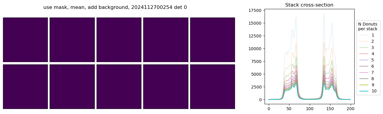

In the above example, with mean and nanmean the stacked pixel count decreases, because we are adding progressively fainter donuts to the average. Next we illustrate the difference between using mask and not using the mask. We only plot a fragment of each donut to highlight the differences:
# illustrate the donuts

add_bkgnd = True
pixel_stack = "nanmean"
for use_mask in [True, False]:

    fig,axs = plt.subplots(2,5, figsize=(10,4))
    ax = np.ravel(axs)
    ax_hist =  fig.add_axes([1.0,0.15,0.3,0.8])
    i = 0
    lines = []
    for n in range(1,11):

        stackedExtra = rs.stack_donut_wep_im_refactor(
            donutStampsExtra,
            n=n,
            pixel_stack=pixel_stack,
            use_mask=use_mask,
            after_avg_fill_with_bkgnd=add_bkgnd,
        )
        mask_string = "use" if use_mask else "no"
        background_string = "add" if add_bkgnd else "no"
        if i < len(ax):


            xmin,xmax = 20,100
            ymin,ymax = xmin,xmax
            ycross = (ymin+ymax)//2
            ax[i].imshow(dummy)
            #ax[i].imshow(stackedExtra['donutStackedArray'][20:100, 20:100], origin='lower',)
            ax[i].axhline(ycross-ymin, c='orange', ls='--')
            ax[i].set_xticks([])
            ax[i].set_yticks([])
            i += 1

        # plot the cross-section
        line = ax_hist.plot(stackedExtra['donutStackedArray'][xmin:xmax, ycross], alpha=n*0.1)
        lines.append(line)
    flat_lines = [line[0] if isinstance(line, list) else line for line in lines]
    ax_hist.legend(handles=flat_lines, labels=[str(n) for n in range(1,11)],
             bbox_to_anchor = [1,0.9],  title='N Donuts \nper stack',)
    ax_hist.set_title('Stack cross-section')
    fig.subplots_adjust(hspace=0.05, wspace=0.05)


    if len(donutStamps)<len(ax):
        for i in range(len(donutStamps), len(ax)):
            ax[i].axis('off')
    fig.suptitle(f"{mask_string} mask, {pixel_stack}, {background_string} background, {visit} det {detector}")


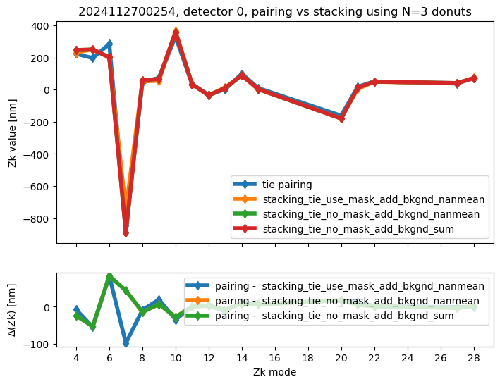
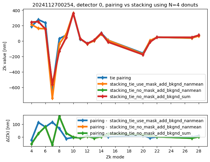
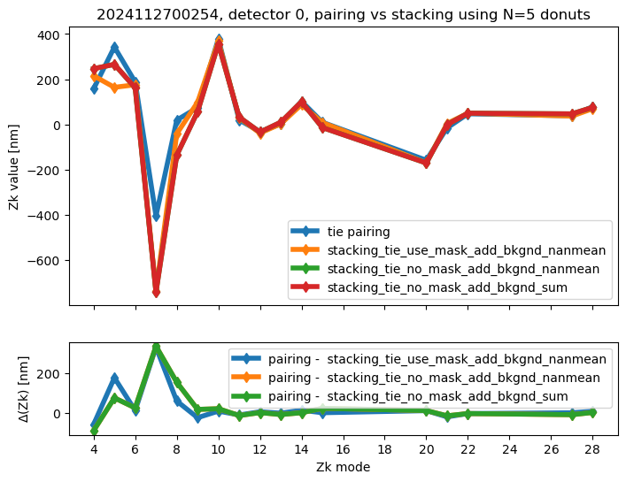
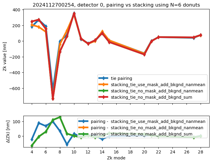
We run stacking with the attached run_stacking.py code for each dataset reference (i.e. visit / detector). Since the results of wavefront fitting are compared against individual pairs that used the following Zk mode sequence: [4, 5, 6, 7, 8, 9, 10, 11, 12, 13, 14, 15, 20, 21, 22, 27, 28], we use exactly the same setting in fitting the stacked results. First we highlight the results of stacking for a single detector:
single_file_results_dir = '/sdf/group/rubin/shared/scichris/DM-47822_stacking_comcam/stacking_per_visit_det_ndonut_new/'
aggregate_results_dir = '/home/s/scichris/link_to_scichris/WORK/sitcomtn-158/'
aggregate_fname = 'stacking_pairing_table_rows_0-1000.txt'
fname = os.path.join(aggregate_results_dir,aggregate_fname)
stacking_pairing = Table.read(fname,format='ascii')
import re
zk_modes  = [4, 5, 6, 7, 8, 9, 10, 11, 12, 13, 14, 15, 20, 21, 22, 27, 28]
method = 'tie'
# A flag so we only plot pairing once
for Ndonuts in range(1,10):
    fig, ax = plt.subplots(2, 1, sharex=True, figsize=(8, 6), gridspec_kw={'height_ratios': [3, 1]})
    not_plotted_pairing = True
    for row in rows:
        if row['ndonuts'] == Ndonuts:
            # pairing method is the same as stacking
            method_stacking = row['method']
            method_pairing = method_stacking.split('_')[1]
            if method  == method_pairing:
                 ### pairing result
                zks = row['zk_pairing']
                # Remove brackets, 'nm', and line breaks
                clean = re.sub(r'[\[\]nm\\n]', '', zks)
                # Convert to numpy array
                arr_pairing = np.fromstring(clean, sep=' ')

                if not_plotted_pairing :
                    ax[0].plot(zk_modes, arr_pairing, marker='d',
                            lw=4, label=f'{method_pairing} pairing')
                    not_plotted_pairing = False
                ### stacking result
                zks = row['zk_stacking']
                # Remove brackets, 'nm', and line breaks
                clean = re.sub(r'[\[\]nm\\n]', '', zks)

                # Convert to numpy array
                arr_stacking = np.fromstring(clean, sep=' ')
                ax[0].plot(zk_modes, arr_stacking, marker='d',
                        lw=4, label=method_stacking)

                # Calculate difference
                diff = arr_pairing - arr_stacking
                ax[1].plot(zk_modes, diff, marker='d',
                        lw=4, label=f'pairing -  {method_stacking}')

                ax[0].set_title(f"{visit}, detector {detector}, pairing vs stacking using N={Ndonuts} donuts")
                ax[0].set_xticks(np.arange(4,29,step=2))
                ax[0].set_ylabel(  'Zk value [nm]', rotation='vertical')
                ax[0].legend()#bbox_to_anchor=[1.0,0.86])
                ax[1].legend()
                ax[1].set_xticks(np.arange(4,29,step=2))
                ax[1].set_xlabel( 'Zk mode')
                ax[1].set_ylabel( r'$\Delta$'+'(Zk) [nm]', rotation='vertical')
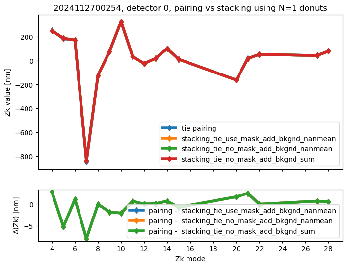
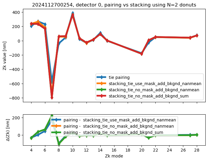
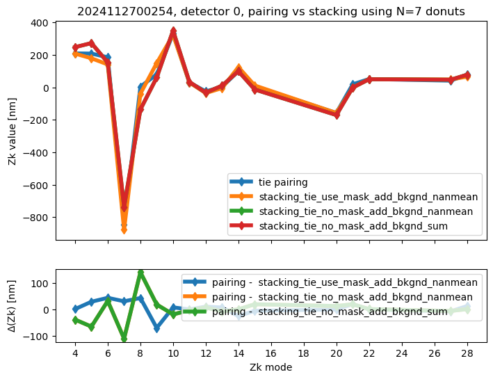
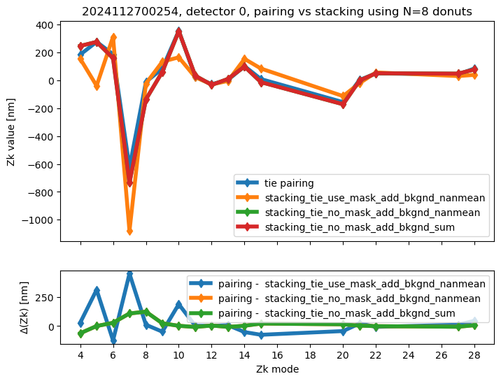
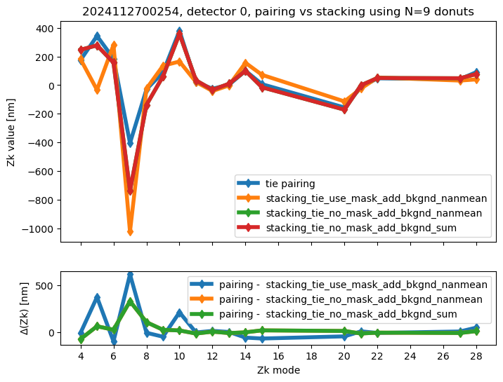
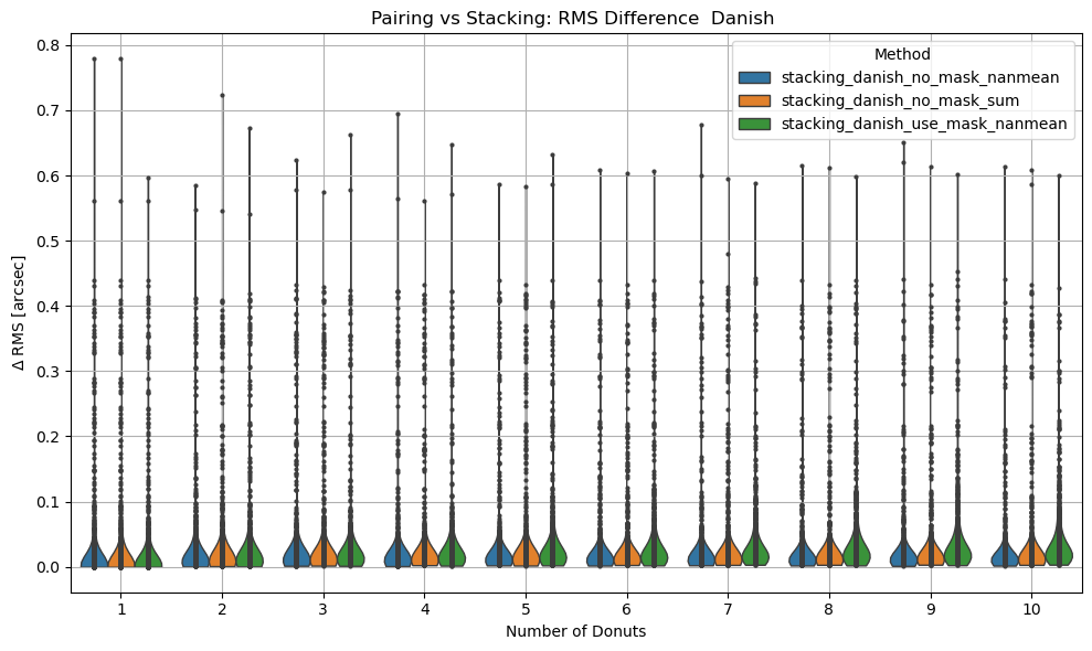
We calculate the RMS difference between $\( \langle zk_{i,P} \rangle_{N} - zk_{i,S,N} \)\( where \)\langle zk_{i,P} \rangle_{N} \( corresponds to mean of pairing results for N donut pairs , while \)zk_{i,S,N}$ to fitting with WEP the stack consisting of the same donuts.
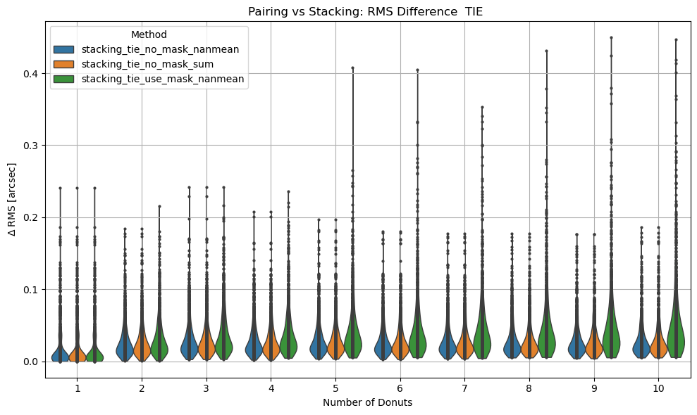
Aggregate plots#
fname = '/home/s/scichris/link_to_scichris/WORK/sitcomtn-158/stacking_pairing_table_rows_0-1000.txt'
stacking_pairing = Table.read(fname,format='ascii')
methods = np.unique(stacking_pairing['method'])
labels = np.char.replace(methods.data, "add_bkgnd_", "")

summary = {}

for chosen in ['tie', 'danish']:

    # Prepare a DataFrame for violinplot
    records = []
    for method in methods:
        if chosen in method:
            label = method.replace("add_bkgnd_", "")
            mask = stacking_pairing['method'].data == method
            rms_diff_asec = np.array([float(value.split()[0]) for value in stacking_pairing[mask]['rms_diff_asec'].data])
            ndonuts = stacking_pairing[mask]['ndonuts'].data

            # Collect records
            for n, rms in zip(ndonuts, rms_diff_asec):
                records.append({
                    'ndonuts': n,
                    'rms_diff_asec': rms,
                    'method': label
                })

    # Convert to DataFrame
    df = pd.DataFrame(records)

    # Plot with seaborn
    plt.figure(figsize=(10, 6))
    sns.violinplot(data=df, x='ndonuts', y='rms_diff_asec', hue='method',density_norm='width', inner='point', cut=0, linewidth=1)

    plt.xlabel('Number of Donuts')
    plt.ylabel(r'$\Delta$ RMS [arcsec]')
    title = 'TIE' if chosen == 'tie' else 'Danish'
    plt.title(f'Pairing vs Stacking: RMS Difference  {title} ')
    plt.grid(True)
    plt.legend(title='Method')
    plt.tight_layout()
    plt.show()

    # calculate what percentage of points are below a given RMS threwhold
    ns = []
    ps = []
    ms = []

    threshold  = 0.07
    for n in range(1,10):
        for method in np.unique(df['method']):
            #print(method)
            mask_class = (df['method'] == method) & (df['ndonuts'] == n)
            mask_thresh = mask_class & (df['rms_diff_asec'] < threshold)
            perc = 100 * np.sum(mask_thresh) / np.sum(mask_class)
            ns.append(n)
            ps.append(perc)
            ms.append(method)
            print(f'For N={n} donuts , {perc} percent are below {threshold} for {method}')

    summary[chosen] = {'ns':ns, 'ps':ps,'ms':ms}
For N=1 donuts , 93.2 percent are below 0.07 for stacking_tie_no_mask_nanmean
For N=1 donuts , 93.2 percent are below 0.07 for stacking_tie_no_mask_sum
For N=1 donuts , 93.2 percent are below 0.07 for stacking_tie_use_mask_nanmean
For N=2 donuts , 92.9 percent are below 0.07 for stacking_tie_no_mask_nanmean
For N=2 donuts , 92.9 percent are below 0.07 for stacking_tie_no_mask_sum
For N=2 donuts , 90.5 percent are below 0.07 for stacking_tie_use_mask_nanmean
For N=3 donuts , 88.6 percent are below 0.07 for stacking_tie_no_mask_nanmean
For N=3 donuts , 88.6 percent are below 0.07 for stacking_tie_no_mask_sum
For N=3 donuts , 84.7 percent are below 0.07 for stacking_tie_use_mask_nanmean
For N=4 donuts , 91.2 percent are below 0.07 for stacking_tie_no_mask_nanmean
For N=4 donuts , 91.2 percent are below 0.07 for stacking_tie_no_mask_sum
For N=4 donuts , 85.7 percent are below 0.07 for stacking_tie_use_mask_nanmean
For N=5 donuts , 90.9 percent are below 0.07 for stacking_tie_no_mask_nanmean
For N=5 donuts , 90.9 percent are below 0.07 for stacking_tie_no_mask_sum
For N=5 donuts , 83.8 percent are below 0.07 for stacking_tie_use_mask_nanmean
For N=6 donuts , 91.5 percent are below 0.07 for stacking_tie_no_mask_nanmean
For N=6 donuts , 91.5 percent are below 0.07 for stacking_tie_no_mask_sum
For N=6 donuts , 82.2 percent are below 0.07 for stacking_tie_use_mask_nanmean
For N=7 donuts , 91.1 percent are below 0.07 for stacking_tie_no_mask_nanmean
For N=7 donuts , 91.1 percent are below 0.07 for stacking_tie_no_mask_sum
For N=7 donuts , 81.2 percent are below 0.07 for stacking_tie_use_mask_nanmean
For N=8 donuts , 91.8 percent are below 0.07 for stacking_tie_no_mask_nanmean
For N=8 donuts , 91.8 percent are below 0.07 for stacking_tie_no_mask_sum
For N=8 donuts , 80.2 percent are below 0.07 for stacking_tie_use_mask_nanmean
For N=9 donuts , 92.4 percent are below 0.07 for stacking_tie_no_mask_nanmean
For N=9 donuts , 92.4 percent are below 0.07 for stacking_tie_no_mask_sum
For N=9 donuts , 78.6 percent are below 0.07 for stacking_tie_use_mask_nanmean
For N=1 donuts , 92.9 percent are below 0.07 for stacking_danish_no_mask_nanmean
For N=1 donuts , 92.9 percent are below 0.07 for stacking_danish_no_mask_sum
For N=1 donuts , 93.6 percent are below 0.07 for stacking_danish_use_mask_nanmean
For N=2 donuts , 93.0 percent are below 0.07 for stacking_danish_no_mask_nanmean
For N=2 donuts , 92.4 percent are below 0.07 for stacking_danish_no_mask_sum
For N=2 donuts , 92.6 percent are below 0.07 for stacking_danish_use_mask_nanmean
For N=3 donuts , 93.6 percent are below 0.07 for stacking_danish_no_mask_nanmean
For N=3 donuts , 92.9 percent are below 0.07 for stacking_danish_no_mask_sum
For N=3 donuts , 94.4 percent are below 0.07 for stacking_danish_use_mask_nanmean
For N=4 donuts , 94.3 percent are below 0.07 for stacking_danish_no_mask_nanmean
For N=4 donuts , 93.9 percent are below 0.07 for stacking_danish_no_mask_sum
For N=4 donuts , 94.2 percent are below 0.07 for stacking_danish_use_mask_nanmean
For N=5 donuts , 94.4 percent are below 0.07 for stacking_danish_no_mask_nanmean
For N=5 donuts , 92.8 percent are below 0.07 for stacking_danish_no_mask_sum
For N=5 donuts , 92.3 percent are below 0.07 for stacking_danish_use_mask_nanmean
For N=6 donuts , 93.8 percent are below 0.07 for stacking_danish_no_mask_nanmean
For N=6 donuts , 93.3 percent are below 0.07 for stacking_danish_no_mask_sum
For N=6 donuts , 91.4 percent are below 0.07 for stacking_danish_use_mask_nanmean
For N=7 donuts , 94.8 percent are below 0.07 for stacking_danish_no_mask_nanmean
For N=7 donuts , 93.1 percent are below 0.07 for stacking_danish_no_mask_sum
For N=7 donuts , 90.9 percent are below 0.07 for stacking_danish_use_mask_nanmean
For N=8 donuts , 94.8 percent are below 0.07 for stacking_danish_no_mask_nanmean
For N=8 donuts , 93.9 percent are below 0.07 for stacking_danish_no_mask_sum
For N=8 donuts , 90.1 percent are below 0.07 for stacking_danish_use_mask_nanmean
For N=9 donuts , 94.7 percent are below 0.07 for stacking_danish_no_mask_nanmean
For N=9 donuts , 93.2 percent are below 0.07 for stacking_danish_no_mask_sum
For N=9 donuts , 89.6 percent are below 0.07 for stacking_danish_use_mask_nanmean
We combine that information on a single plot, serving as a summary of what percentage of all considered donut stacks are below a given RMS threshold
fig,ax = plt.subplots(1,1,figsize=(7,5))
for me in summary.keys():
    for method in np.unique(summary[me]['ms']):
        m = np.array(summary[me]['ms']) == method
        marker='o'
        if me == 'tie':
            marker='s'
        ax.scatter(np.array(summary[me]['ns'])[m]
                    , np.array(summary[me]['ps'])[m], label=method,
                    marker=marker
               )
ax.legend()
ax.set_xlabel("N donuts")
ax.set_ylabel("% of sample below RMS threshold")
ax.set_title(f'Points below RMS of {threshold} asec')
Text(0.5, 1.0, 'Points below RMS of 0.07 asec')
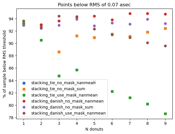
This shows that for a given number of donuts, differences between each stacking method are very small.
Include exposure-level information and seeing#
client = ConsDbClient('http://consdb-pq.consdb:8080/consdb')
print(f'schemas:\n', client.schema())

schema = 'lsstcomcam'
table = 'exposure'
print(f'columns (table={table}): {table} \n',
      list(client.schema('lsstcomcam', f'cdb_{schema}.{table}').keys()
          )
      )

query = f"""
SELECT *
from cdb_lsstcomcam.exposure e
where  e.img_type = 'CWFS'
and e.day_obs between 20241025 and 20241212
--order by e.seq_num desc
"""
df = client.query(query)
schemas:
 ['latiss', 'lsstcam', 'lsstcamsim', 'lsstcomcam', 'lsstcomcamsim', 'startrackerfast', 'startrackernarrow', 'startrackerwide']
Select a subset that corresponds to visits with the stacking-pairing results;
# Table that has the same length as pairing stacking information
visit_det = stacking_pairing[['visit', 'det']]


df_sub = df[np.isin(df['exposure_id'], np.unique(visit_det['visit']))]
For these visits, given the time of beginning and end of each exposure, we add information from Gemini about seeing.
seeing_dt = []
seeing = []
with open("../sitcomtn-158/gemini_complete.txt") as file:
    for row in file:
        if row[0] == "#" or row == "\n":
            continue
        if "Channel" in row:
            continue
        date, time, *_, s = [item for item in row.split(" ") if item != ""]
        digits = [int(float(item)) for item in date.split("/") + time.split(":")]
        seeing_dt.append(datetime(*digits) + timedelta(hours=3))
        seeing.append(float(s.strip("\n")))

seeing_dt = np.array(seeing_dt)
seeing = np.array(seeing)

idx = seeing_dt.argsort()
seeing_dt = seeing_dt[idx]
seeing = seeing[idx]

# mask out bad values

mask = seeing < 100
seeing_dt = seeing_dt[mask]
seeing = seeing[mask]

seeing_mjd = Time(seeing_dt).mjd
We initially test if there’s seeing data within the exposure time. If there isn’t, we expand the search window by 1 min increments, until a maximum of 10 mins is reached.
one_min_mjd = 1 / 1440        # 1 minute in MJD
max_min = 10
max_expansion = max_min * one_min_mjd  # 5 minutes in MJD

seeing_found = []
seeing_window = []
for i in range(len(df_sub)):
    mjd_start = df_sub[i]['obs_start_mjd']
    mjd_end = df_sub[i]['obs_end_mjd']
    initial_end = mjd_end  # store original end

    mask = (mjd_start < seeing_mjd) & (seeing_mjd < mjd_end)

    # Expand window if no matches
    while np.sum(mask) == 0 and (mjd_end - initial_end) < max_expansion:
        mjd_end += one_min_mjd
        mask = (mjd_start < seeing_mjd) & (seeing_mjd < mjd_end)
    if np.sum(mask) > 0:
        #print(i, np.sum(mask), f"(final end: {mjd_end})")
        seeing_found.append(np.median(seeing[mask]))
    elif np.sum(mask) == 0:
        #print(f"No seeing data found for index {i} even after {max_min}-minute expansion.")
        seeing_found.append(np.nan)
    seeing_window.append(mjd_end-mjd_start)
df_sub['seeing_gemini'] = seeing_found
df_sub['seeing_window'] = seeing_window
Now we can add this information to the pairing-stacking results:
# Obtain relevant info from consDB - Gemini exposure table via a join
visit_det_mjd = join(left=visit_det,  right=df_sub, keys_left='visit',
                     keys_right='exposure_id',
                     join_type='left')
Within a given stacking method and a number of donuts, plot the dependence of \(\Delta RMS \) from Gemini seeing:
visit_det_mjd[:3]
| visit | det | exposure_id | exposure_name | controller | day_obs | seq_num | physical_filter | band | s_ra | s_dec | sky_rotation | azimuth_start | azimuth_end | azimuth | altitude_start | altitude_end | altitude | zenith_distance_start | zenith_distance_end | zenith_distance | airmass | exp_midpt | exp_midpt_mjd | obs_start | obs_start_mjd | obs_end | obs_end_mjd | exp_time | shut_time | dark_time | group_id | cur_index | max_index | img_type | emulated | science_program | observation_reason | target_name | air_temp | pressure | humidity | wind_speed | wind_dir | dimm_seeing | focus_z | simulated | s_region | vignette | vignette_min | seeing_gemini | seeing_window |
|---|---|---|---|---|---|---|---|---|---|---|---|---|---|---|---|---|---|---|---|---|---|---|---|---|---|---|---|---|---|---|---|---|---|---|---|---|---|---|---|---|---|---|---|---|---|---|---|---|---|---|---|
| int64 | int64 | int64 | str20 | str1 | int64 | int64 | str4 | str4 | float64 | float64 | float64 | float64 | float64 | float64 | float64 | float64 | float64 | float64 | float64 | float64 | float64 | str26 | float64 | str26 | float64 | str26 | float64 | float64 | float64 | float64 | str26 | int64 | int64 | str4 | bool | str12 | object | str23 | float64 | float64 | float64 | float64 | float64 | object | float64 | object | object | str9 | str9 | float64 | float64 |
| 2024102700034 | 2 | 2024102700034 | CC_O_20241027_000034 | O | 20241027 | 34 | r_03 | r | 1.1772020363064675 | -69.00569211567523 | 335.4250271565598 | 173.527696953535 | 173.603695504982 | 173.5656962292585 | 50.844358275922 | 50.8577731705796 | 50.8510657232508 | 39.155641724078 | 39.1422268294204 | 39.1489342767492 | 1.2888126838829248 | 2024-10-28T01:36:38.447000 | 60611.06711165439 | 2024-10-28T01:36:23.227000 | 60611.06693549953 | 2024-10-28T01:36:53.667000 | 60611.067287809245 | 30.0 | 30.0 | 30.439558506011963 | 2024-10-28T01:35:39.170#1 | 1 | 1 | CWFS | False | BLOCK-T160 | EXTRA_manual_alignment | 14.399999618530273 | 74435.0 | 9.675000190734863 | 2.9189999103546143 | 21.23998260498047 | None | 2.133299113086085 | None | None | UNKNOWN | UNKNOWN | 0.664777502852 | 0.00035230971116106957 | |
| 2024102700034 | 2 | 2024102700034 | CC_O_20241027_000034 | O | 20241027 | 34 | r_03 | r | 1.1772020363064675 | -69.00569211567523 | 335.4250271565598 | 173.527696953535 | 173.603695504982 | 173.5656962292585 | 50.844358275922 | 50.8577731705796 | 50.8510657232508 | 39.155641724078 | 39.1422268294204 | 39.1489342767492 | 1.2888126838829248 | 2024-10-28T01:36:38.447000 | 60611.06711165439 | 2024-10-28T01:36:23.227000 | 60611.06693549953 | 2024-10-28T01:36:53.667000 | 60611.067287809245 | 30.0 | 30.0 | 30.439558506011963 | 2024-10-28T01:35:39.170#1 | 1 | 1 | CWFS | False | BLOCK-T160 | EXTRA_manual_alignment | 14.399999618530273 | 74435.0 | 9.675000190734863 | 2.9189999103546143 | 21.23998260498047 | None | 2.133299113086085 | None | None | UNKNOWN | UNKNOWN | 0.664777502852 | 0.00035230971116106957 | |
| 2024102700034 | 2 | 2024102700034 | CC_O_20241027_000034 | O | 20241027 | 34 | r_03 | r | 1.1772020363064675 | -69.00569211567523 | 335.4250271565598 | 173.527696953535 | 173.603695504982 | 173.5656962292585 | 50.844358275922 | 50.8577731705796 | 50.8510657232508 | 39.155641724078 | 39.1422268294204 | 39.1489342767492 | 1.2888126838829248 | 2024-10-28T01:36:38.447000 | 60611.06711165439 | 2024-10-28T01:36:23.227000 | 60611.06693549953 | 2024-10-28T01:36:53.667000 | 60611.067287809245 | 30.0 | 30.0 | 30.439558506011963 | 2024-10-28T01:35:39.170#1 | 1 | 1 | CWFS | False | BLOCK-T160 | EXTRA_manual_alignment | 14.399999618530273 | 74435.0 | 9.675000190734863 | 2.9189999103546143 | 21.23998260498047 | None | 2.133299113086085 | None | None | UNKNOWN | UNKNOWN | 0.664777502852 | 0.00035230971116106957 |
methods = np.unique(stacking_pairing['method'])
fig,ax = plt.subplots(1,1,figsize=(7,4))
for n in range(10):
    method = methods[0]
    # choose rows only for that method and number of donuts stacked
    mask = (stacking_pairing['method'].data == method) & (stacking_pairing['ndonuts'].data == n)

    rms_diff_asec = np.array([float(value.split()[0]) for value in stacking_pairing[mask]['rms_diff_asec'].data])
    ndonuts = stacking_pairing[mask]['ndonuts'].data

    seeing = visit_det_mjd[mask]['seeing_gemini']

    ax.scatter(seeing, rms_diff_asec, s=15, alpha=0.75, label = n )
ax.set_xlim(-.05,2.1)
ax.legend(title='N donuts')
ax.set_ylabel(r'$\Delta$ RMS [arcsec]')
ax.set_xlabel(r' Gemini seeing [arcsec]')
Text(0.5, 0, ' Gemini seeing [arcsec]')
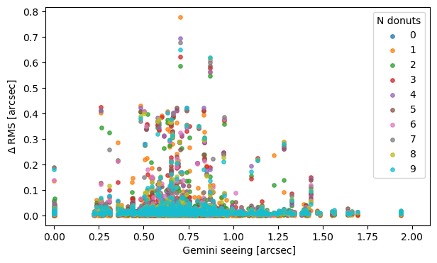
We don’t see a clear trend of eg. higher RMS being more likely with the larger seeing value.
Summary#
We observe that the pairing vs. stacking results are notably robust across stacking methods, particularly when using the Danish algorithm. In 94% of cases, the total RMS difference remains at or below 0.07 arcseconds. The TIE algorithm shows similarly stable behavior, with 96% of cases falling below this threshold when stacking 10 donuts without applying mask information. Overall, TIE without masking performs comparably to Danish, regardless of whether masking is applied, indicating that the choice of stacking method has limited impact on the final RMS for these configurations.